What is Simulink
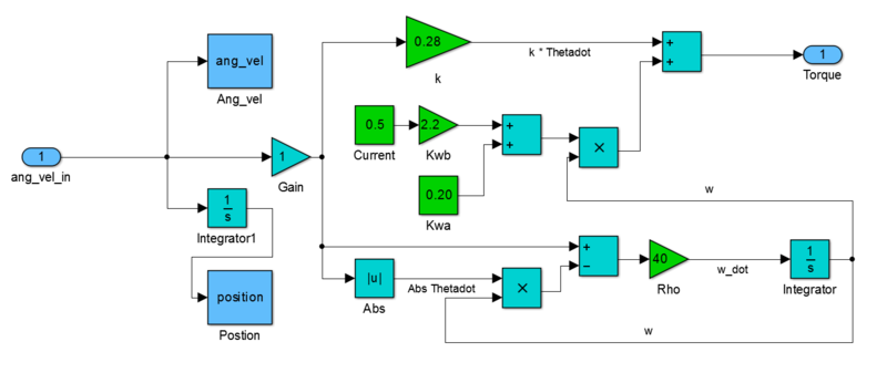
Image Credit: Sangle445 / CC BY-SA. commons.wikimedia.org
Simulink is a simulation and design environment provided by MATLAB® provided by MathWorks. It is primarily used for simulating and analysing multidomain dynamical systems by using a graphical block diagramming user interface into which the user can assemble a functional model by connecting programmable blocks which are made available from within several domain specific libraries.
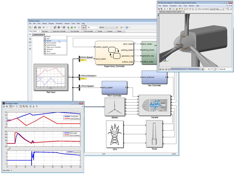
Image Credit: Mcarone1 / CC BY-SA. commons.wikimedia.org
Simulink is widely used in physical modelling, signal processing and in the design or testing of automatic control systems, but a more comprehensive knowledge of of its extensive domain application potential can be seen by reviewing its block libraries:
.
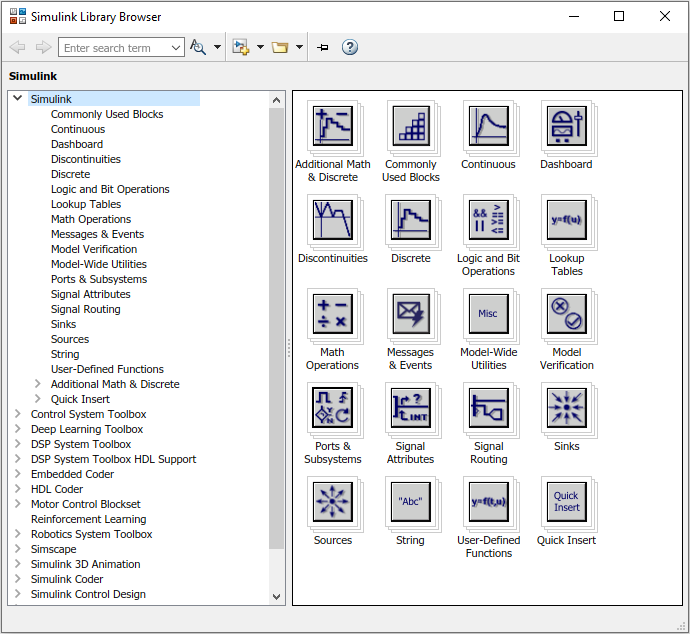
Image Credit: Doug Rattray, UHI.
Simulink is tightly intergrated into the MATLAB® environment enabling the user to export simulation results to MATLAB for further analysis or to drive Simulink from within MATLAB. When driven from within MATLAB, Simulinks capabilities are extended further by enabling block parameter assignment, the use of coded algorithms and the scheduling of multiple consequtive simulations for contingency analyses.
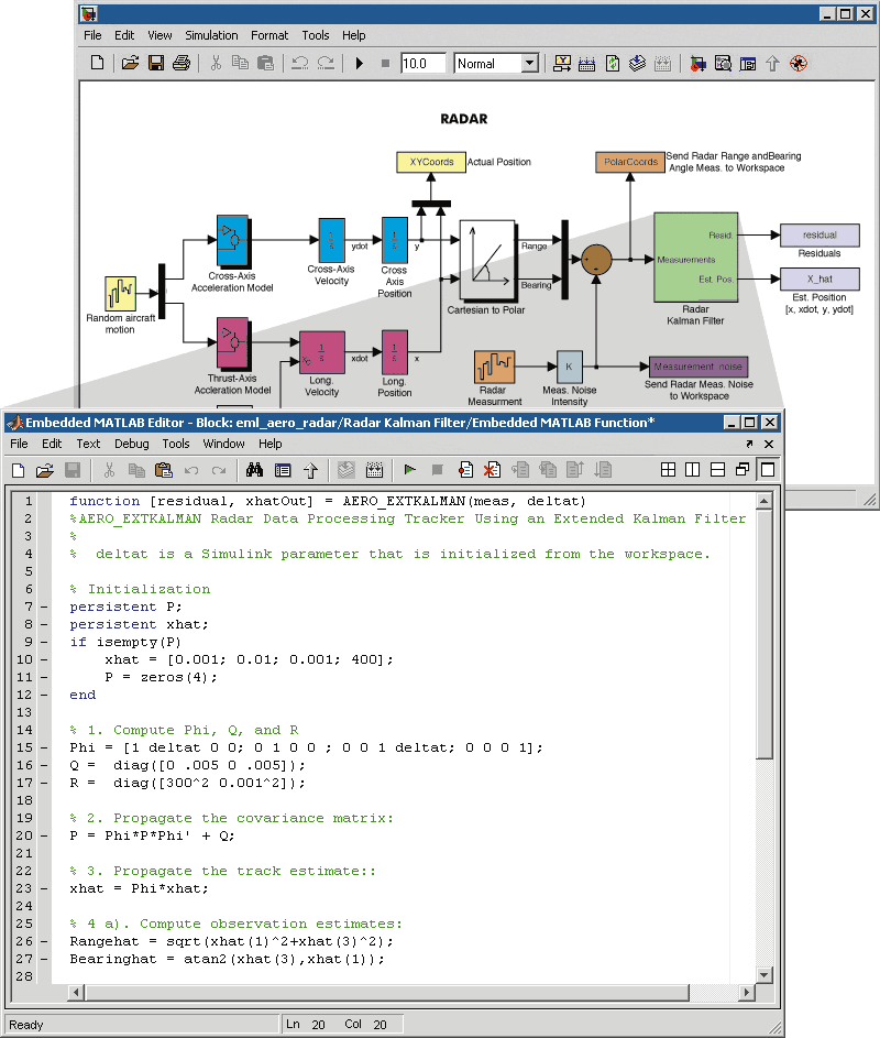
Image Credit: GustavatoR / Public domain. commons.wikimedia.org
How to Access MATLAB® Simulink
Creating a MathWorks Account
Note: if you already have a MathWorks Account in the format your_student_ID@uhi.ac.uk you can use that account and skip this step.

Image Credit: Doug Rattray, UHI.
- Use your student email address to register
- Select ‘Student Use’ in the ‘How will you use MathWorks software?’ field
- Confirm you are over 13 and click on ‘Create’
- You will be sent an email from service@mathworks.com to verify your account
- The link in the email will take you to a page to complete your personal details.
- Complete your profile details entering "the university of highlands and islands" as your institution.
Installing the Application
- Once you have completed your account setup, your licence details should be displayed as 'MATLAB (Individual)' and you should be prompted to 'Use MATLAB Online' or 'Install MATLAB'.
- Select 'Install MATLAB' to begin the installation.
- Note you may wish to check the system requirements for your machine when selecting a version to download.
- Open the Installed application and select 'Log in with a MathWorks Account' entering your unveristy email address login credentials.
- Continue through the setup and select 'Install'.
Troubleshooting
If at any stage of the installation process, you are having trouble, contact the service desk for assistance.
- Telephone: 01463 279150
- Email: servicedesk@uhi.ac.uk
- Live Chat: https://uhi.bomgarcloud.com/
Learning Resources
MathWorks provide a high quality online resource for learning the basics of how to create, edit and simulate models in Simulink. The course takes approximately three hours to complete and is free to access at the following link.
https://uk.mathworks.com/learn/tutorials/simulink-onramp.html
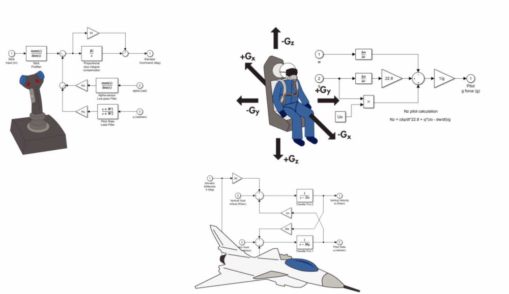
Image Credit: Doug Rattray, UHI.
The course content consists of interactive course lessons on the following subjects:
- Course Overview
- Simulink Graphical Environment
- Inspecting Signals
- Basic Algorithms
- Obtaining Help
- Project: Automotive Performance Modes
- Simulink and MATLAB
- Dynamic Systems in Simulink
- Discrete Systems
- Continuous Systems
- Simulation Time
- Project: Modelling a Thermostat
- Project: Peregine Falcon Dive
In addition MATLAB provide a comprehensive set of instructional videos demonstrating its application in many domains on their youtube channel:
https://www.youtube.com/user/MATLAB

Image Credit: Doug Rattray, UHI.
The Simulink Software Environment
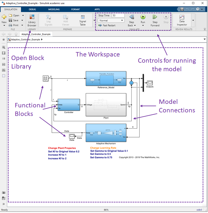
Image Credit: Doug Rattray, UHI.
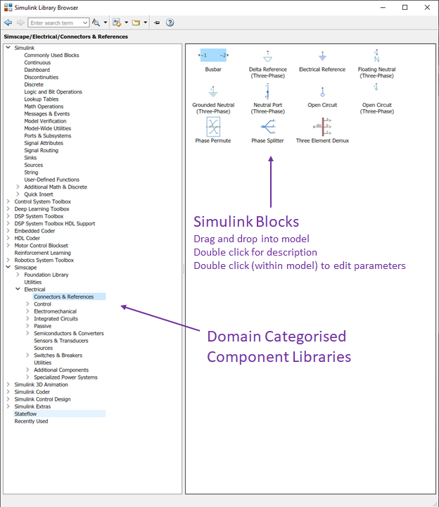
Image Credit: Doug Rattray, UHI.
Examples
MathWorks provides an extensive suite of examples that users can explore. These are accessible through the simulink startup page.
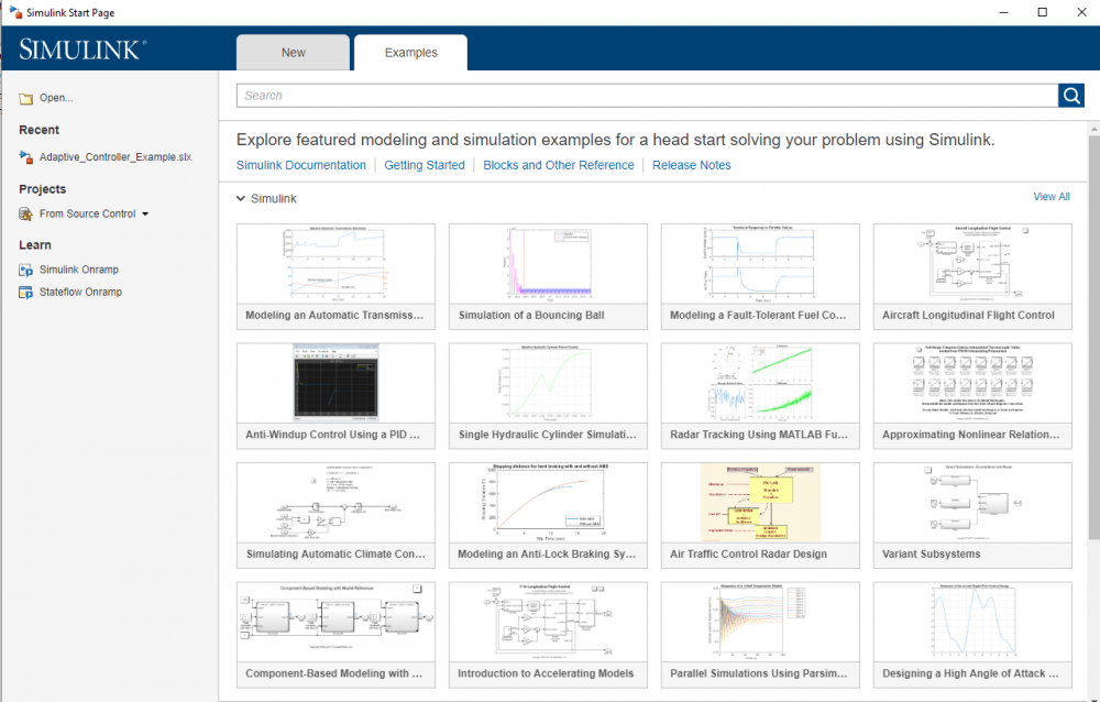
Image Credit: Doug Rattray, UHI.
Walkthrough
MATLAB Simulink provides a toolset for modelling and simulating the generation, transmission, distribution, and consumption of electrical power. In this class we shall:
- Explore the blocks of the Simscape Electrical Specialised Power System Library;
- Learn how to build a single phase transmission system model by bringing these blocks into the Simulink workspace;
- Learn about the Powergui block and how it is used to define our Simulation Solver;
- Interconnect blocks to create our circuit and run our simulation;
- Bring in and configure various measurement blocks to view the results of our simulation.
Our Single Phase Transmission System
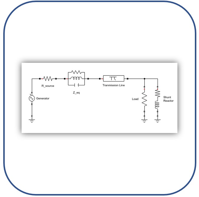
The circuit illustrated in the figure below represents an equivalent power system feeding a 300 km transmission line. The line feeds a static load at its receiving end and is also provided with voltage compensation by means of a shunt reactor. A circuit breaker allows us to switch the circuit in or out of service, i.e., to energise or de-energise the line.
The parameters selected here are arbitrary but in any case representative of typical 400 kV transmission system.

Figure: Single Phase Transmission System
Creating the Model
- To open Simulink, at the MATLAB Command Window, enter: ‘simulink’
- Select to open a blank model and save the new model as: ‘Simple_SL_Transmission_System.slx’.
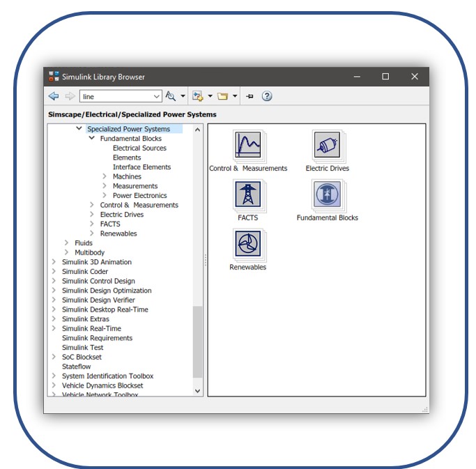
- Open the Library Browser and navigate the tree structure to:
- Simscape / Electrical / Specialised Power Systems
- Note: you can open a browser direct to this block library by entering the command ‘simpowersystems_ST’ into the MATLAB Command Window.
- This library contains many of the blocks that we shall be use to build our model.
Modelling the Generator
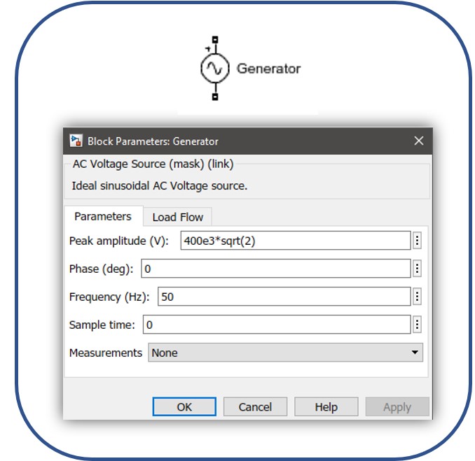
- Add an ‘AC Voltage Source’ block to the model by dragging and dropping the block into the workspace.
- Simscape / Electrical / Specialised Power Systems / Fundamental Blocks / Electrical Sources
- By clicking on the block name, rename it to: ‘Generator’.
- By double-clicking on the AC Voltage Source block within the model, set the parameters for the block as shown in our circuit diagram.
- Note: this block requires peak amplitude of voltage to be input, i.e., a 400 kV RMS voltage should be entered as ‘400e3*sqrt(2)’.
Modelling the Generator Impedance
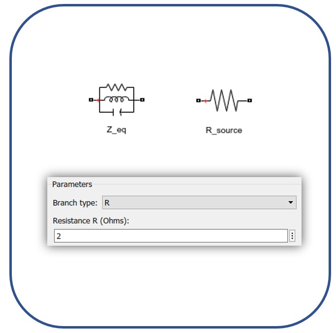
- Add a ‘Parallel RLC Branch’ block to the model, rename to ‘Z_eq’ and set the parameters in accordance with our circuit diagram.
- Simscape / Electrical / Specialised Power Systems / Fundamental Blocks / Elements
- Add a second ‘Parallel RLC Branch’ block (or copy the one above), rename to ‘R_source’ and set the parameters in accordance with our circuit diagram.
- Change Branch Type from ‘RLC’ to ‘R’ if the block is only to model resistive elements. Note that the inductive and capacitive icons in the block disappear once this change has been applied.
- HINT: blocks can be copied quickly pressing (and holding) the CTRL key, click and drag upon the existing block and drag to a new location.
Modelling the Generator Connections
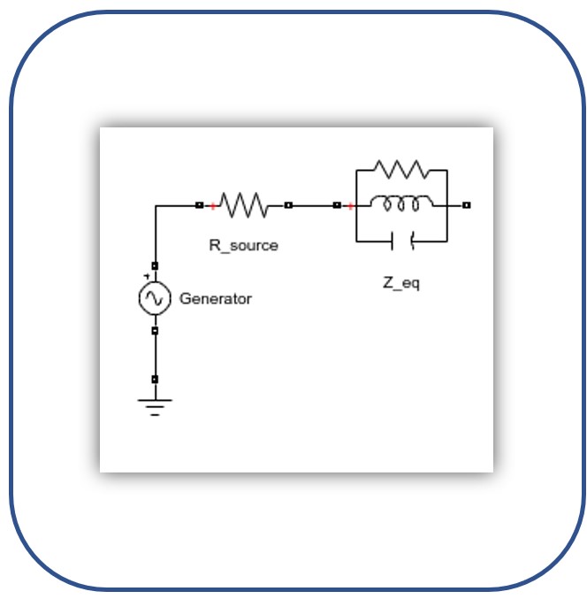
- Add a ‘Ground’ block to the model.
- Simscape / Electrical / Specialised Power Systems / Fundamental Blocks / Elements
- Resize and re-position the blocks to your preference.
- By dragging lines between the terminals of each block, make the connections between blocks in accordance with our circuit diagram.
- Note that these connections act as lines or cables in a power system but have zero impedance.
- To model line and cable impedance, specific blocks need to be brought into the model to represent those components.
Modelling the Transmission Line
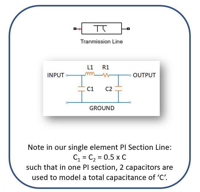
- Add a ‘PI Section Line’ block to the model, rename to ‘Transmission Line’ and set the parameters in accordance with our circuit diagram.
- Simscape / Electrical / Specialised Power Systems / Fundamental Blocks / Elements
- A transmission line with uniformly distributed RLC parameters results in a time delay due to wave propagation along the line. We cannot model this continuously as the delay corresponds to an infinite number of states. However the PI Section Line allows us to simulate a good approximation of this using a finite number of cascading PI circuits (discrete elements) each representing a small section of the line.
- Each PI Section consists of a series RL branch with two shunt C branches. The model accuracy (and run time) depends on the number of PI sections stipulated for the model.
Modelling the Load and Shunt Reactor
- Add two ‘Series RLC Load’ blocks to the model, rename to ‘Load’ and ‘Shunt Reactor’ and set the parameters in accordance with our circuit diagram.
- Simscape / Electrical / Specialised Power Systems / Fundamental Blocks / Elements
- Note that the Series Load Block allows you to specify the active and reactive powers directly instead of the RLC parameters (see ‘Series RLC Branch’ block).
The quality factor allows us to calculate the absorbed power of the shunt reactor: (P = Q/k)
- Add the required ‘Ground’ blocks to the model and connect all of our elements in accordance with the circuit diagram.
- Note that at present we are omitting the circuit breaker. This shall be considered at a later stage.
The Powergui Block
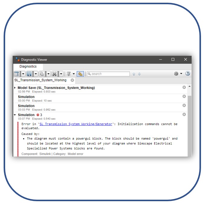
The final requirement is to configure the solver. To do so, we add the ‘powergui’ block to the model.
- Simscape / Electrical / Specialised Power Systems / Fundamental Blocks
The powergui block is the environment block for Simscape Electrical Specialized Power Systems models. It is used to store the equivalent Simulink circuit that represents the state-space equations of Specialised Power System blocks.
The powergui block offers various tools for specific analyses (such as FFT Analysis) and preferences that can be modified to for advanced parameter design or model initialisation.
The powergui block allows us to choose one of these methods for solving our model:
- Continuous, utilising a variable step solver
- Discrete, utilising a fixed step solver
- Phasor, solving the phase space equations
We may return to some of these settings later but for now we can leave this block set to it’s default ‘Continuous’ type simulation and solve our model.

Running our Model
To run the model press the run simulation button illustrated below:
![]()
Shortcut key stroke: CTRL + T
If there are any errors in the model, the Diagnostic Viewer window will automatically display them.
Further information on troubleshooting using the Diagnostic Viewer can be found at:
Once our model has successfully solved we are able to start viewing the results of our simulation. This will require some additional measurement blocks to be added into the model.
Measuring Voltage
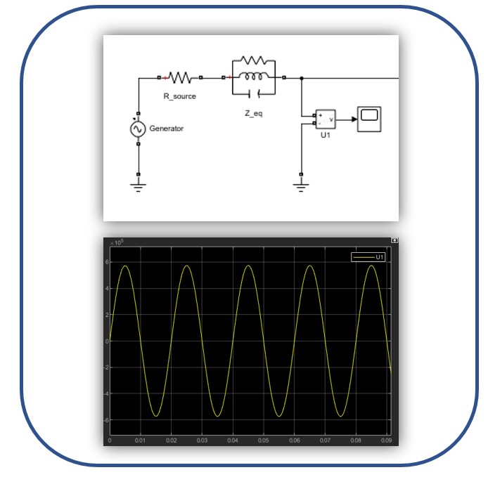
- Add a ‘Voltage Measurement’ block to the model, rename to ‘U1’ and connect the positive terminal to the output of our generator equivalent circuit. Connect the negative terminal to a ‘Ground’ block.
- Simscape / Electrical / Specialised Power Systems / Fundamental Blocks / Measurements
- To visualise this voltage, a display system is required. Connect a ‘scope’ block to the output of the voltage measurement as illustrated.
- Simulink / Sinks
Run the simulation again. Double click on the scope block to view the results. The scope block will automatically adjust the axis scale to fit the results. Explore each of the various zooming tools in the toolbar so that you can visualise the AC voltage waveform.
- Simulink / Sinks
Comparing Transmission Line Voltages
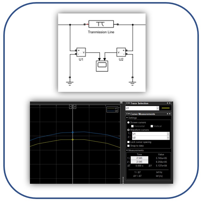
- Add a second ‘Voltage Measurement’ block to the model, rename to ‘U2’ and connect the positive terminal to the end of our transmission line.
- Connect the output of this second measurement block to the same scope.
- Note that the scope should add an additional terminal automatically but if it does not the number of input ports can be configured by right clicking on the scope and selecting the number of inputs from within ‘signals and ports’.
Run the simulation again. Open the scope and adjust the axis scale so that you can view the voltage drop along the line. Explore the use of the cursor measurement tool in the toolbar so that you can quantify the change in peak AC voltage.
- Note that the scope should add an additional terminal automatically but if it does not the number of input ports can be configured by right clicking on the scope and selecting the number of inputs from within ‘signals and ports’.
Measuring Current
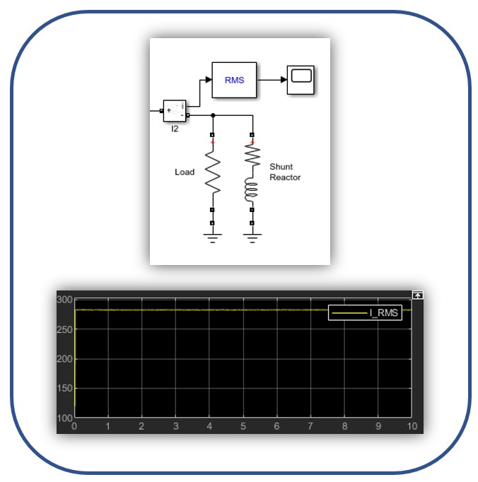
- Add a ‘Current Measurement’ block to the model, rename to ‘I2’ and connect it in series to the output of our transmission line as illustrated.
- Simscape / Electrical / Specialised Power Systems / Fundamental Blocks / Measurements
- To view the RMS current add an ‘RMS’ and ‘Scope’ block to the model and connect to the output of the current measurement block.
- …Specialised Power Systems / Control & Measurements / Measurements
Run the simulation again. Double click on the scope block to view the results.
- …Specialised Power Systems / Control & Measurements / Measurements
Summary
This module has provided a short introduction to the MATLAB® Simulink software environment, which allows for the simulation and design of systems accross many desciplines of engineering.
This module has only touched upon the vast capabilities and applications of this toolset. MATLAB® Simulink is employed extensively both in academia and industry and gaining good knowledge & understanding of the toolset would be of great benefit to aspiring students.


